SQL Practice

library(tidyverse)
library(mdsr)
library(dbplyr)
library(DBI)

# connect to the scidb server on Amazon Web Services - the airlines 
# database lives on a remote server
db <- dbConnect_scidb("airlines")
flights <- tbl(db, "flights")
planes <- tbl(db, "planes")

On Your Own - Extended Example from MDSR

Refer to Section 15.5 in MDSR, where they attempt to replicate FiveThirtyEight’s plot of slowest and fastest airports in the section below Figure 15.1. Instead of using target time, which has a complex definition, we will use arrival time, which oversimplifies the situation but gets us in the ballpark.

The MDSR authors provide a mix of SQL and R code to perform their analysis, but the code will not work if you simply cut-and-paste as-is into R. Your task is to convert the book code into something that actually runs. [Hint: use dbGetQuery()]

On Your Own - Practice with SQL

These problems are based on class exercises from MSCS 164 in Fall 2023, so you’ve already solved them in R! Now we’re going to try to duplicate those solutions in SQL.

# Read in 2013 NYC flights data
library(nycflights13)

Warning: package 'nycflights13' was built under R version 4.3.3


Attaching package: 'nycflights13'

The following objects are masked _by_ '.GlobalEnv':

    flights, planes

flights_nyc13 <- nycflights13::flights
planes_nyc13 <- nycflights13::planes

Summarize carriers flying to MSP by number of flights and proportion that are cancelled (assuming that a missing arrival time indicates a cancelled flight). [This was #4 in 17_longer_pipelines.Rmd.]

# Original solution from MSCS 164
flights_nyc13 |>
  mutate(carrier = fct_collapse(carrier, "Delta +" = c("DL", "9E"), 
                                      "American +"= c("AA", "MQ"), 
                                     "United +" = c("EV", "OO", "UA"))) |>
  filter(dest == "MSP") |>   
  group_by(origin, carrier) |>
  summarize(n_flights = n(), 
            num_cancelled = sum(is.na(arr_time)),
            prop_cancelled = mean(is.na(arr_time)))

`summarise()` has grouped output by 'origin'. You can override using the
`.groups` argument.

# A tibble: 5 × 5
# Groups:   origin [3]
  origin carrier    n_flights num_cancelled prop_cancelled
  <chr>  <fct>          <int>         <int>          <dbl>
1 EWR    Delta +          598            10         0.0167
2 EWR    United +        1779           105         0.0590
3 JFK    Delta +         1095            41         0.0374
4 LGA    Delta +         2420            25         0.0103
5 LGA    American +      1293            62         0.0480

First duplicate the output above, then check trends across all years and origins. Here are a few hints:

use flights instead of flights_nyc13
remember that flights_nyc13 only contained 2013 and 3 NYC origin airports (EWR, JFK, LGA)
is.na can be replaced with CASE WHEN arr_time = ‘NA’ THEN 1 ELSE 0 END
CASE WHEN can also be used replace fct_collapse

SELECT carrier, dest, arr_time, origin, year,
  SUM(1) AS n_flights, 
  SUM(CASE WHEN arr_time  = 'NA' THEN 1 ELSE 0 END) as num_cancelled, 
  AVG(CASE WHEN arr_time  = 'NA' THEN 1 ELSE 0 END) as prop_cancelled, 
  CASE WHEN (carrier = 'DL' OR carrier = 'E9') THEN 'Delta +'
       WHEN (carrier = 'AA' OR carrier = 'MQ') THEN 'American +'
       WHEN (carrier = 'EV' OR carrier = 'OO' OR carrier = "UA") THEN 'United +'
       ELSE 'Other' END AS new_carrier
FROM flights
WHERE dest = "MSP" AND year = 2013 AND (origin = "EWR" OR origin = "JFK" OR origin = "LGA")
GROUP BY origin, new_carrier
ORDER BY prop_cancelled DESC;

8 records
carrier	dest	arr_time	origin	year	n_flights	num_cancelled	prop_cancelled	new_carrier
EV	MSP	800	EWR	2013	1779	105	0.0590	United +
MQ	MSP	847	LGA	2013	1293	62	0.0480	American +
9E	MSP	954	JFK	2013	1070	41	0.0383	Other
9E	MSP	1310	EWR	2013	178	5	0.0281	Other
DL	MSP	1007	EWR	2013	420	5	0.0119	Delta +
DL	MSP	751	LGA	2013	2419	25	0.0103	Delta +
DL	MSP	1018	JFK	2013	25	0	0.0000	Delta +
9E	MSP	2225	LGA	2013	1	0	0.0000	Other

Plot number of flights vs. proportion cancelled for every origin-destination pair (assuming that a missing arrival time indicates a cancelled flight). [This was #7 in 17_longer_pipelines.Rmd.]

# Original solution from MSCS 164
res2 <- flights_nyc13 |>
  group_by(origin, dest) |>
  summarize(n = n(),
            prop_cancelled = mean(is.na(arr_time))) |>
  filter(prop_cancelled < 1)

`summarise()` has grouped output by 'origin'. You can override using the
`.groups` argument.

res2

# A tibble: 223 × 4
# Groups:   origin [3]
   origin dest      n prop_cancelled
   <chr>  <chr> <int>          <dbl>
 1 EWR    ALB     439        0.0478 
 2 EWR    ANC       8        0      
 3 EWR    ATL    5022        0.0271 
 4 EWR    AUS     968        0.00930
 5 EWR    AVL     265        0.0453 
 6 EWR    BDL     443        0.0700 
 7 EWR    BNA    2336        0.0385 
 8 EWR    BOS    5327        0.0146 
 9 EWR    BQN     297        0.00673
10 EWR    BTV     931        0.0473 
# ℹ 213 more rows

res2 |>  ggplot(aes(n, prop_cancelled)) + 
  geom_point()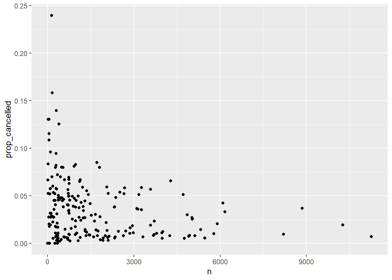

SELECT origin, dest, arr_time,
    SUM(1) AS n, 
    AVG(CASE WHEN arr_time  = 'NA' THEN 1 ELSE 0 END) AS prop_cancelled
FROM flights
WHERE year = 2013 AND (origin = "EWR" OR origin = "JFK" OR origin = "LGA") 
GROUP BY origin, dest
HAVING prop_cancelled < 1

res2sql |>  ggplot(aes(n, prop_cancelled)) + 
  geom_point()

First duplicate the plot above, then check trends across all years and origins. Do all of the data wrangling in SQL. Here are a few hints:

use flights instead of flights_nyc13
remember that flights_nyc13 only contained 2013 and 3 NYC origin airports (EWR, JFK, LGA)
use an sql chunk and an r chunk
include connection = and output.var = in your sql chunk header (this doesn’t seem to work with dbGetQuery()…)

Produce a table of weighted plane age by carrier, where weights are based on number of flights per plane. [This was #6 in 26_more_joins.Rmd.]

# Original solution from MSCS 164
flights_nyc13 |>
  left_join(planes_nyc13, join_by(tailnum)) |>
  mutate(plane_age = 2013 - year.y) |>
  group_by(carrier) |>
  summarize(unique_planes = n_distinct(tailnum),
            mean_weighted_age = mean(plane_age, na.rm =TRUE),
            sd_weighted_age = sd(plane_age, na.rm =TRUE)) |>
  arrange(mean_weighted_age)

# A tibble: 16 × 4
   carrier unique_planes mean_weighted_age sd_weighted_age
   <chr>           <int>             <dbl>           <dbl>
 1 HA                 14              1.55            1.14
 2 AS                 84              3.34            3.07
 3 VX                 53              4.47            2.14
 4 F9                 26              4.88            3.67
 5 B6                193              6.69            3.29
 6 OO                 28              6.84            2.41
 7 9E                204              7.10            2.67
 8 US                290              9.10            4.88
 9 WN                583              9.15            4.63
10 YV                 58              9.31            1.93
11 EV                316             11.3             2.29
12 FL                129             11.4             2.16
13 UA                621             13.2             5.83
14 DL                629             16.4             5.49
15 AA                601             25.9             5.42
16 MQ                238             35.3             3.13

First duplicate the output above, then check trends across all years and origins. Do all of the data wrangling in SQL. Here are a few hints:

SELECT f.carrier, COUNT(DISTINCT f.tailnum) AS unique_planes, avg((2013 - p.year)) AS mean_weighted_age, STDDEV(2013 - p.year) AS sd_weighted_age 
FROM flights AS f
LEFT JOIN planes AS p ON f.tailnum = p.tailnum
WHERE f.year = 2013 AND f.year != 'NA' AND (origin = "EWR" OR origin = "JFK" OR origin = "LGA") 
GROUP BY f.carrier
ORDER BY mean_weighted_age;

Displaying records 1 - 10
carrier	unique_planes	mean_weighted_age	sd_weighted_age
HA	14	1.5484	1.137022
AS	84	3.3366	3.068823
VX	53	4.4736	2.135061
F9	26	4.8787	3.665043
B6	193	6.6867	3.289461
OO	28	6.8438	2.373149
9E	204	7.1011	2.669565
US	290	9.1037	4.881782
WN	583	9.1461	4.625865
YV	58	9.3138	1.925773

use flights instead of flights_nyc13
remember that flights_nyc13 only contained 2013 and 3 NYC origin airports (EWR, JFK, LGA)
you’ll have to merge the flights dataset with the planes dataset
you can use DISTINCT inside a COUNT()

dbDisconnect(db)